The E-Value in Regression: A Useful, Simple, Easily Understood, and Easily Applied Statistic

For Readers Unfamiliar With Concepts in Statistics

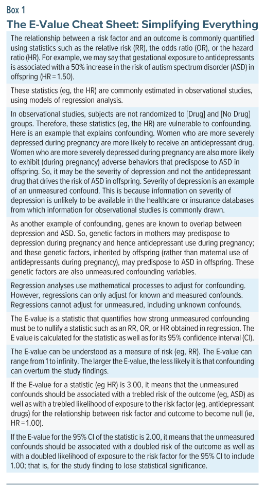
Readers may find it helpful to study the cheat sheet presented in Box 1. The cheat sheet simplifies the contents of this article and, once understood, should make it easier to navigate through the text that follows.

As with all articles on statistics, it is advisable to read slowly, assimilate text, and re-read text for best assimilation of content.

Readers who already have adequate knowledge about risk, confidence intervals, confounding, and regression will find the contents of this article easy to assimilate. Readers who wish to improve their knowledge about these subjects may wish to consult the references cited in the Supplementary Material accompanying this article.

Introductory Notes

Observational studies commonly examine whether a risk factor is associated with an adverse outcome. When the data are analyzed using regression and related methods to adjust for covariates and confounds, the result is a statistic such as the odds ratio (OR) or the hazard ratio (HR).

We now face the question: how robust are these ORs and HRs against bias from residual confounding; or, more specifically, against bias arising from unmeasured, including unknown confounds? This is an important question because the purpose of an ideally adjusted regression analysis is to identify the unique, unconfounded association between the risk factor and the adverse outcome. This is a particularly important question when cause-effect relationships are being considered.

As a side note here, whereas adjusting for confounds usually lowers the unadjusted risk, when suppressor variables are also adjusted for, adjustment can result in an increase in the value of the risk. The latter result was obtained, for example, in a cohort study of pregabalin and major congenital malformations (MCMs)¹ when secondary analyses compared pregabalin with other treatments. So, whereas incompletely addressed confounding is more usually associated with higher values of risk, it may occasionally be associated with lower values.

As another side note, residual confounding, referred to above, arises from many sources, including unknown confounds, unmeasured confounds, imperfectly measured confounds, and an imperfectly specified regression model (eg, a model that does not include important interactions). In this article, unmeasured confounding is used for convenience because this is the term that is widely used in the context of the E-value.

These side notes are both relevant to discussions about the E-value, later in this article.

A Research Question

Consider a real example, discussed in an earlier article in this column.² We want to know whether gestational exposure to acetaminophen is associated with an increased risk of autism spectrum disorder (ASD). We should ideally address this question in a randomized controlled trial (RCT). However, an RCT in pregnancy may be ethically problematic, would require a very large sample because ASD is an uncommon outcome, and would require many years of follow-up to ensure that all subjects with ASD are identified in the sample.

What alternatives do we have? We can use observational data from insurance and healthcare databases. Disadvantages of using observational data are that data on many important covariates and confounds may not be available, data on those that are available may not have been accurately measured and recorded, and diagnoses of ASD may not have been rigorously made. Additionally, there could be considerable exposure misclassification because we cannot know whether women advised and dispensed acetaminophen actually took the drug, or whether women obtained acetaminophen over the counter and took it without its use being recorded in the database. Advantages of using observational data are that insurance and healthcare databases contain information on hundreds of thousands of subjects, and that data with long-term follow-up are immediately available. This list of advantages and disadvantages is not comprehensive.

When RCTs are unavailable or unfeasible, we use observational study designs to search for answers to our research question. Case-control and cohort studies provide us with information, in the form of ORs and HRs, about the association between gestational exposure to acetaminophen and ASD in offspring. We now return to the question raised earlier in this article: how robust are these ORs and HRs against bias arising from unmeasured, including unknown confounds? This is where the E-value is of help.

The E-Value

An earlier article in this column³ presented the fragility index for RCTs; this is the smallest number of subjects in the RCT whose outcome status needs to be changed, such as from remitted to unremitted, for a statistically significant test result to lose its statistical significance. In similar manner, the E-value is the smallest strength of an unmeasured confound that could bring a significant risk value (relative risk [RR], OR, or HR) to the null value, or at least to statistical nonsignificance.

The E-value was introduced by VanderWeele and Ding.⁴ These authors defined the E-value as the “minimum strength of association, on the risk ratio scale, that an unmeasured confounder would need to have with both the treatment and the outcome to fully explain away a specific treatment-outcome association, conditional on the measured covariates.” This definition is explained in the following sections, using a real example.

As a side note here, for readers who may be curious, the E in E-value does not have an expansion; at least, the authors did not provide one.⁴

As another side note, the E-value can be considered as a hypothetical effect size (RR, OR, or HR, as relevant to the study) necessary for unmeasured confounding to nullify the observed estimate.

The Example

Ahlqvist et al⁵ found that gestational exposure to acetaminophen was associated with a significantly increased risk of ASD in crude (HR, 1.26; 95% confidence interval [CI], 1.22–1.29) as well as in fully adjusted (HR, 1.05; 95% CI, 1.02–1.08) analyses; the E-value was 1.28 for the adjusted HR (ie, 1.05) and 1.16 for the lower bound of its 95% CI (ie, 1.02).

Readers may note that, in this study, although the adjusted HR was small, it was statistically significant. The conclusion that we draw is that even after the authors adjusted for all (known and measured) covariates and confounds, gestational exposure to acetaminophen remained associated with a small but significantly increased risk of ASD.

Two Questions

We know that, in their study,⁵ the authors would not have been able to adjust their analyses for the many genetic and environmental risk factors for ASD.⁶ We have a gut feeling that their statistically significant HR of 1.05 could easily have been brought down to the null value of 1.00 had these unmeasured risk factors been taken into account. A reasonable question, therefore, is “How strong should the unmeasured confounding have been to nullify the observed HR?” The E-value is the answer to this question.

There are actually 2 E-values that address our question. One is the E-value for the adjusted estimate of risk (HR = 1.05), and the other is the E-value for the lower bound of its 95% CI (HR = 1.02). The former E-value answers the question, “How strong should the unmeasured confounding be to bring the HR from 1.05 to 1.00?” The latter E-value answers the question, “How strong should the unmeasured confounding be to bring the lower bound of the HR from 1.02 to 1.00; that is, into the statistically nonsignificant range?” For those to whom statistical significance is important, it is the latter E-value that is more important.

The Answers

As already stated, Ahlqvist et al⁵ found that the E-value was 1.28 for the adjusted HR (1.05) and 1.16 for the lower bound of its 95% CI (1.02). This means that if there is an unmeasured confound with a strength of association of 1.28 (or higher) with both acetaminophen and ASD, its inclusion in the regression would lower the HR for the association between acetaminophen and ASD from 1.05 to the null value of 1.00.

With regard to the second E-value, if the unmeasured confound had a strength of association of as little as 1.16 with both acetaminophen and ASD, its inclusion in the regression would bring the lower bound of the 95% CI from 1.02 to the null value of 1.00. That is, the association between acetaminophen and ASD would no longer be statistically significant because the 95% CI includes the null value.

Additional explanatory notes about the E-value are provided in the sections that follow.

How Is the E-Value for the Estimate Calculated?

Calculation of the E-value is ridiculously simple and can easily be done by the researcher, reviewer, editor, and even reader. The only information required to calculate the E-value is the estimate (eg, the RR, OR, or HR) that was obtained in the study. No additional information is required. This means that the numerical value of the E-value depends only on the numerical value of the estimate, and is independent of study design, sample size, covariates included in the regression, 95% CI of the estimate, and other details.

For an RR value of 1.00 or higher, the formula for the E-value is⁴:

E= RR + square root of [RR(RR−1)]

For an HR value of 1.00 or higher, the formula is the same, except that we insert the HR in place of RR in the formula.

As a worked example for HR = 1.05, the derivation is:

E= 1.05 + square root of [1.05(1.05–1)]

This simplifies to 1.05 + 0.23, or 1.28; the same value that was stated by Ahlqvist et al⁵ in the study cited earlier.

For an OR value of 1.00 or higher, when the outcome is uncommon (eg, prevalence <15% in the population), the formula is the same, except that we insert the OR in place of RR in the formula.

For the OR, if the outcome is common (eg, prevalence >15% in the population), the OR meaningfully overestimates the RR, and using the formula shown above would result in an inflated E-value. A different formula is applied; because this derivation of the E-value is more complex, it is not further explained here, but interested readers may refer to the explanation provided by VanderWeele and Ding.⁴

If the RR, HR, or OR are <1.00, the same formula is used, except that the value input in the formula is the reciprocal of the RR, HR, or OR. So, if the OR for an uncommon outcome is 0.50, the reciprocal of 0.50 (that is, 2.00) is input in the formula, and the E-value obtained is 3.41.

The E-value can also be estimated for outcomes such as mean difference and risk difference; the procedures were described by VanderWeele and Ding.⁴

The Value of the E-Value

From the preceding section, it is apparent that the E-value is always a positive number. The E-value can lie anywhere between 1 and infinity. An E-value of 1 means that no unmeasured confound needs to be present to bring the estimate to null. Larger E-values mean that unmeasured confounding needs to be stronger to nullify the estimate.

How Is the E-Value for the 95% CI Calculated?

The E-value for the 95% CI is sought by those to whom the statistical significance of the estimate is important. It is usual to calculate the E-value for only the lower bound of the 95% CI when the RR, OR, or HR is >1.00 and for only the upper bound of the 95% CI when the estimate is <1.00. This is because the purpose of estimating the E-value of the 95% CI is to determine the strength of confounding required to bring that limit of the CI to 1.00; that is, to bring the null value into the CI, thereby making the estimate no longer statistically significant. No useful information is obtained by calculating the E-value for the other limit of the CI.

As an example, in the study by Ahlqvist et al,⁵ the 95% CI was 1.02–1.08. We’re interested in the E-value only of the lower bound; that is, we want to know the strength of confounding that would bring 1.02 to 1.00. Knowing the E-value of the upper bound, 1.08, conveys no useful information to us.

There is no need to calculate the E-value for the 95% CI if the 95% CI already includes 1.00. This is because there is no unmeasured confounding necessary to make the estimate statistically nonsignificant; it is already nonsignificant.

The same formula, used to calculate the E-value for an estimate, stated in a previous section, is used to calculate the E-value for the CI. The value input in the formula is the lower bound of the CI when the value is >1.00 and the reciprocal of the upper bound of the CI when the value is <1.00.

Calculating the E-Value, Simplified

Given that only the value of the estimate (RR, OR, HR) is required to calculate the E-value, it should immediately be apparent that for a given value of an estimate, the E-value is a fixed number. So, E-value tables are available online, as are E-value calculators. These can be identified from a simple online search for “E-value table” or “E-value online calculator,” pasted into a browser search box without the quotation marks.

Here is one of many online calculators: https://www.evalue-calculator.com/ (accessed on January 9, 2026).

This website provides instructions on how to use the calculator, and it allows the calculation of the E-value for different kinds of estimate for different prevalences of the outcome in the population. It also provides the E-value for the CI and a plot that decomposes the E-value into different values for strength of association with risk factor and outcome (see the next section for the explanation).

It is preferable to use an E-value calculator rather than a table of E-values because the calculator provides more options.

Decomposing the E-Value

The E-value is the least strength of association that the unmeasured confound should have with both the risk factor and the outcome. So, if the E-value is 2, after accounting for measured covariates, the RR between the unmeasured confound and the risk factor should be at least 2.00, and the RR between the unmeasured confound and the outcome should also be at least 2.00.

On the surface, this seems to be a somewhat unreasonable specification. However, there is a very good reason for it. If the unmeasured confound has a low strength of association with the risk factor, it would need to have a high to very high strength of association with the outcome to be able to bring the estimate to null. Or, if the unmeasured confound has a low strength of association with the outcome, it will need to have a high to very high strength of association with the risk factor to be able to bring the estimate to null.

Both of the scenarios described above are unlikely. It is also quite inconvenient to present the reader with a multitude of E-value pairs, one for each strength of association of the confound with the risk factor along with its corresponding strength of association with the outcome. So, the solution proposed by VanderWeele and Ding⁴ was eminently sensible; the E-value is the smallest single value for strength of association between the unmeasured confound and the risk factor as well as between the unmeasured confound and the outcome, required to bring the estimate to null.

The message here is that the single-value E-value was chosen for convenience. The E-value can also be represented by paired values; that is, a smaller value for one association along with a larger value for the other association. The online calculator, referenced in the previous section, effortlessly generates the required plot of paired values for any given value of the estimate.

The Unmeasured Confound

In an earlier section, we calculated that if a risk factor is associated with an RR (or OR, HR) of 0.50 (or 2.00), the E-value is 3.41. This is a very large value for a strength of association of an unmeasured confound with both risk factor and outcome. If such a strong risk factor existed, chances are that it would not be unknown and hence unmeasured.

Readers may note that the larger the E-value, the less likely it is that unmeasured confounding exists to nullify the finding. However, this observation depends on whether adjustment for confounds has already been extensive; if adjustment has been minimal to modest, many unadjusted confounds may exist for even a high E-value to be plausible.

Whether adjustment for confounding has been moderate or extensive, it is necessary to consider whether the existence of additional confounding is plausible. Judgment depends on how large the E-value is along with what is known in the field.

The E-value does not assume that the confounding should arise from a single unmeasured confound. It can arise from a composite of all unmeasured confounding, including confounding from imperfectly measured confounds, unmeasured and unknown confounds, and interactions that were not specified in the regression model; in other words, residual confounding, which is a bit more than merely unmeasured confounding.

How does this operate in real studies? Lee et al⁷ found that in each of the 3 trimesters of pregnancy, exposure to antidepressant medications was associated with a significantly increased risk of ASD; the adjusted HRs lay in the 1.35 to 1.46 range. A quick calculation tells us that the E-value for 1.46 is 2.28. So, the unmeasured confound would need to have a more than doubled strength of association with both antidepressant exposure and the ASD outcome. Such a strong unmeasured confound, or composite confound, probably did exist, because the same study obtained very similar HRs for ASD in prepregnancy antidepressant exposure analysis and in paternal antidepressant exposure analysis; furthermore, in this study, the HR in discordant sibling pair analysis was not statistically significant. All these findings suggest that confounding, rather that gestational exposure to antidepressants, drove the ASD risk in offspring. A single unmeasured confound is unlikely; it is more probable that genetic, family environment, and maternal illness risk factors put together constituted a composite confound that sufficed to explain the association between antidepressant exposure and ASD.⁸ So, a high E-value does not rule out unmeasured confounding.

The plausibility of unmeasured confounding does not depend only on the magnitude of the E-value. It also depends on whether the researchers, and readers, have an idea of what the unmeasured confound(s) may be. In the study by Lee et al,⁷ it was confounding by indication, made up of genetic, family environment, and maternal illness risk factors.

A low E-value does not rule out a causal relationship between the risk factor and the outcome. This is true even if the existence of unmeasured confounding is plausible and candidate variables for confounding are known. Likelihood of confounding is not proof of confounding.

It is not sufficient to suggest what the unmeasured confound must be; one must also know that the unmeasured confound is sufficiently prevalent in the population (from which the sample was drawn) for the confound to plausibly explain the results. As an example, in a hypothetical study of gestational exposure to antidepressant drugs and the risk of MCMs in offspring, if the E-value for antidepressant exposure is 1.50, and if exposure to valproate had not been adjusted for, one might speculate that valproate, a known risk factor for MCMs, may be the unmeasured confound. However, this speculation is not appropriate if use of valproate in women was rare in that population.

Reporting and interpreting E-values, including consideration of the existence of the unmeasured confound(s), should be done in the context of considering the known strength of association of known risk factors with the outcome under study.

Finally, when positing the role of unmeasured confounds, due consideration must be paid to the existence of suppressor variables that were not adjusted for and that might weaken the effect of the unmeasured confounds; reference to such a scenario was made at the beginning of this article.

A Matter of Context

The E-value for a risk factor is not set in stone; it depends on the characteristics of the sample as well as on the covariates and confounds adjusted for. A moment’s reflection explains why this is obvious. The E-value is specific for a given value of an RR, OR, or HR. The value of the RR, OR, or HR depends on sample characteristics; the estimate may be higher in some samples, lower in others. Furthermore, the value of the estimate depends on the covariates and confounds that are adjusted for. This is why the E-value is context-specific and should be interpreted only in the context of the sample and the variables adjusted for. This is also why identical E-values have different interpretations in different studies.⁹

It is necessary to remember that the unmeasured confounds represented by the E-value exclude the confounds already adjusted for; therefore, readers must know what variables have been adjusted for.

The more competent and extensive the adjustment, the less plausible it is that unmeasured confounding exists to support an estimated E-value. This assessment depends on an understanding of the field and hence knowledge of what has not been adjusted for. This assessment does not depend on mere numbers of variables adjusted for.

The E-Value in RCTs

Estimating the E-value for RRs in RCTs is reasonable as a sensitivity test for imperfect randomization in small samples; and, regardless of sample size, it is also reasonable as a measure of postrandomization bias (eg, due to inequalities in rescue medicine use, or inequalities in dropout rates). In the former situation, the E-value tells us how strong chance imbalances (at baseline) between groups would need to be to nullify the findings obtained. In the latter situation, the E-value tells us how strong the postrandomization biases would need to be to nullify the findings obtained.

Miscellaneous Notes

This article focused on the application of the E-value in the context of gestational exposure to acetaminophen and ASD in offspring; that is, a risk factor and an adverse outcome. The E-value can also be applied when the exposure is a treatment and the outcome is favorable. For example, in a retrospective cohort study, Cheng et al¹⁰ found that, in adults with type 2 diabetes mellitus, relative to treatment initiation with a dipeptidyl peptidase-4 inhibitor drug, treatment initiation with a glucagon-like peptide-1 receptor agonist was associated with a lower risk of new-onset epilepsy at 5 years (HR 0.82; 95% CI, 0.76–0.88). The E-value for the HR is 1.74, and that for the upper bound of the 95% CI is 1.53.

The E-value has been criticized,¹¹ defended,^9,12 discussed,^13–15 and expanded.¹⁶ The E-value has also been suggested for use in meta-analysis.¹⁷ Interested readers may follow the cited references.

The E-value should not be regarded as the only way to examine bias in an observational study. As with all statistics that summarize data and the results of analyses, the best way to regard the E-value is to consider it as an additional resource to help us understanding study findings.⁹

Parting Notes

The E-value is a simple, easy to calculate, and easy to apply statistic that helps us understand how strong an unmeasured single or composite confound must be to nullify, or at least to render statistically nonsignificant, an adjusted estimate of risk in regression. Interpretation of the E-value should be based on the plausibility of existence of the unmeasured confound(s) and the prevalence of the confound(s) in the population.

E-values, surprisingly, are not commonly reported. They should be reported by researchers, requested by reviewers and editors, and calculated by readers to understand the robustness of statistically significant adjusted estimates against unmeasured confounding.

Article Information

Published Online: February 11, 2026. https://doi.org/10.4088/JCP.26f16324
© 2026 Physicians Postgraduate Press, Inc.
To Cite: Andrade C. The E-value in regression: a useful, simple, easily understood, and easily applied statistic. J Clin Psychiatry. 2026;87(1):26f16324.
Author Affiliations: Department of Clinical Psychopharmacology and Neurotoxicology, National Institute of Mental Health and Neurosciences, Bangalore, India; Department of Psychiatry, Kasturba Medical College, Manipal Academy of Higher Education, Manipal, India.
Corresponding Author: Chittaranjan Andrade, MD, Department of Clinical Psychopharmacology and Neurotoxicology, National Institute of Mental Health and Neurosciences, Bangalore 560029, India ([email protected]).
Relevant Financial Relationships: None.
Funding/Support: None.
Supplementary Material: Available at Psychiatrist.com.